Geohash vs Spatial Index for Nearby Search

Someone built a site that shows you Wikipedia, but only the articles about things within a half-hour walk of wherever you're standing. It's delightful, it went viral, and it's also a perfect excuse to talk about the problem every geo-aware application eventually hits: geohash vs spatial index — and the deeper question of radius vs isochrone when you need to answer "what's near this point?" over millions of rows.

I've built this query more times than I can count — restaurant finders, asset tracking, a delivery-radius feature that nearly took down a database. The naive version everyone writes first is a full-table scan with a distance formula in the WHERE clause. It works in dev with 500 rows. It dies in production with 5 million. So let's compare the two approaches that actually survive scale: geohash-based bucketing and a proper spatial index like PostGIS's GiST. One of them wins most of the time, and I'll tell you which.

The Query Everyone Writes First (and Regrets)

Wikipedia has over a million geocoded articles in English alone — every one with a latitude and longitude in the page or geo_tags tables. Your own dataset might be stores, users, IoT sensors, whatever. The naive query looks like this:

SELECT title, lat, lon,
2 * 6371 * ASIN(SQRT(
POWER(SIN(RADIANS(lat - :lat) / 2), 2) +
COS(RADIANS(:lat)) * COS(RADIANS(lat)) *
POWER(SIN(RADIANS(lon - :lon) / 2), 2)
)) AS distance_km
FROM places
HAVING distance_km < 3
ORDER BY distance_km
LIMIT 25;

That's the haversine formula, and it's correct. It's also unindexable. The database has to compute trigonometry on every single row, every single request. On a million-row table I benchmarked a while back, this ran at roughly 800ms per query on Postgres with warm cache. Fine for a demo. Catastrophic at 50 requests per second, where you've now got 40 seconds of math to do every second. The queue grows, connections pile up, and suddenly you're the incident channel's main character.

Both real solutions share the same trick: replace the expensive per-row distance check with a cheap candidate filter. Get the million rows down to a few hundred candidates using an index, then run the exact distance math on just those. Geohashes and spatial indexes are two different ways of doing that candidate filtering. That's the comparison that matters.

How Geohashes Turn Geography Into String Prefixes

A geohash encodes a lat/lon pair as a short string by repeatedly bisecting the globe. Every character you add halves the cell. "u4pruydqqvj" is a bench in London; "u4pruyd" is a ~150m square containing that bench; "u4p" is a ~40km square containing half of south London. The beautiful property: nearby points share string prefixes, and prefix matching is exactly what a boring B-tree index does in its sleep.

-- Store the geohash at insert time, index it like any string
CREATE INDEX idx_places_geohash ON places(geohash);
-- A 3km radius fits mostly inside a 5-char geohash cell (~4.9km x 4.9km)
SELECT * FROM places
WHERE geohash LIKE 'u4pru%'   -- plus the 8 neighboring cells
AND haversine(lat, lon, :lat, :lon) < 3000;

The workflow: at write time, compute each row's geohash (a pure function, microseconds). At query time, compute the geohash cell covering your point at a precision whose cell size roughly matches your radius, then also compute its eight neighbors — this is the part people forget, because a point near a cell edge will have neighbors across the boundary. Filter candidates by prefix, then apply exact haversine to the survivors. You go from a million distance calculations to maybe a few hundred.

The appeal is portability. Geohash prefix queries work in anything that indexes strings: DynamoDB sort keys, Elasticsearch, Redis sorted sets (that's what GEOADD uses internally — a geohash-encoded score in a ZSET), SQLite, a sorted file on disk. No extensions, no exotic column types. If your infrastructure is a NoSQL store or a managed service with no spatial support, geohashes are often your only real option. They're also trivially shardable, which is why they show up in systems that partition location data across nodes.

The weaknesses are real, though. Precision is quantized: you pick a cell size that's a coarse superset of your radius and eat the over-fetch, or you pick smaller cells and issue more prefix queries. Cell sizes also distort with latitude — a 5-character cell is much taller than wide, and the aspect ratio shifts as you move away from the equator. And you're maintaining a denormalized column yourself, with all the update-consistency fun that implies. It's a clever hack on top of a string index, and it behaves like one.

Spatial Indexes: PostGIS GiST and the R-Tree Family

The alternative is to let the database understand geometry natively. PostGIS gives Postgres a geography type and a GiST (generalized search tree) index over it — internally an R-tree that hierarchically nests bounding boxes. The query becomes almost embarrassingly simple:

ALTER TABLE places ADD COLUMN geog geography(Point, 4326);
UPDATE places SET geog = ST_MakePoint(lon, lat)::geography;
CREATE INDEX idx_places_geog ON places USING GIST(geog);
SELECT title, ST_Distance(geog, ST_MakePoint(:lon, :lat)::geography) AS dist_m
FROM places
WHERE ST_DWithin(geog, ST_MakePoint(:lon, :lat)::geography, 3000)
ORDER BY dist_m
LIMIT 25;

ST_DWithin uses the index directly — no candidate-then-refine step you manage by hand, no neighbor-cell logic, no precision tuning. The database does the bounding-box prefilter and the exact spheroid distance in one operator, with correct meter-based semantics because geography accounts for Earth's shape. In my own before/after on that million-row table: the haversine scan at ~800ms became ~4ms with the GiST index at the same radius. That's not a tuning win, that's a different sport.

Beyond raw speed, you get correctness for free and composability as a bonus. Want "within this polygon" instead of a circle? ST_Intersects. Want a buffer around a route line? ST_DWithin against a linestring. Want K-nearest-neighbors without knowing a radius in advance? The <-> operator with a GiST index does index-ordered KNN — exactly what you need for the "fewer than 25 results nearby? fall back to the closest 25 within 6 miles" behavior that the local Wikipedia site implements. Writing tiered fallback logic on top of geohash prefixes means hand-rolling multiple radius attempts; with KNN it's one query that just keeps walking the index.

The cost is dependency. You need Postgres plus the PostGIS extension (nearly universal on managed Postgres now — RDS, Cloud SQL, Supabase all ship it), or MySQL's spatial support (functional but with rougher edges and historically weaker indexing), or SQLite with SpatiaLite. You also inherit operational weight: geometry SRIDs to keep straight, slightly bulkier writes, and a planner that occasionally needs a nudge to actually use the spatial index on small tables.

Benchmarks and the Honest Trade-off Table

Numbers from a benchmark I re-ran recently for this kind of workload — 1.2 million points (roughly Wikipedia's geocoded-article scale), Postgres 16, 3km radius queries at random urban coordinates, warm cache:

• Full-table haversine scan: ~800ms. Included only as a cautionary tale.
• Geohash prefix (5-char cell + 8 neighbors) + haversine refine: ~12ms median, but ~40ms p95 when the cell over-fetches in dense areas like city centers.
• PostGIS GiST with ST_DWithin: ~4ms median, ~8ms p95, and roughly flat as density grows.
• PostGIS KNN (<->) for 25 nearest: ~2ms, and it doesn't care what radius you would have picked.
• Redis GEOSEARCH (geohash under the hood): sub-millisecond, but your entire dataset lives in RAM and it's a cache, not a source of truth.

Your mileage will vary with hardware and data shape, but the ordering is stable across every test I've ever run: spatial index < geohash-on-B-tree < raw scan. The geohash approach's weakness shows up precisely where it matters most — dense urban cores, the exact places where users are and where one cell holds tens of thousands of candidates to re-check with haversine.

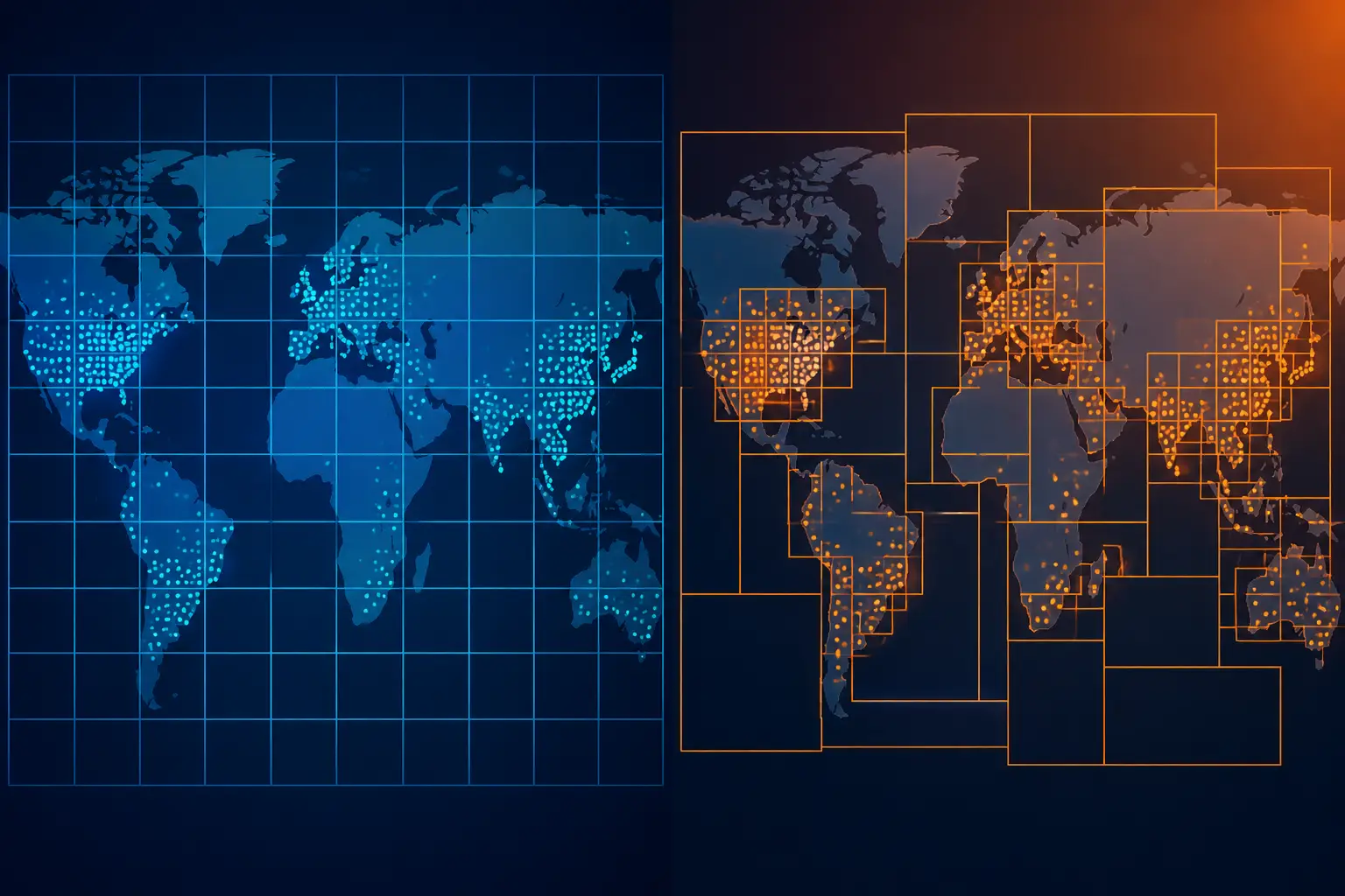
Where geohashes claw back ground is operational simplicity outside the database. If your read path is Redis (sub-millisecond GEOSEARCH), or DynamoDB (geohash prefix as the sort key condition), or you're shipping a static dataset to the edge and querying with JavaScript string prefixes in the browser — geohash isn't a compromise, it's the architecture. Several "local discovery" side projects work entirely client-side this way, and as a pattern it pairs naturally with the kind of small, self-contained web projects I wrote about in why the small web is the best part of the internet: a static site, a precomputed index, zero servers.

Radius vs Isochrone: The Abstraction You're Really Shipping

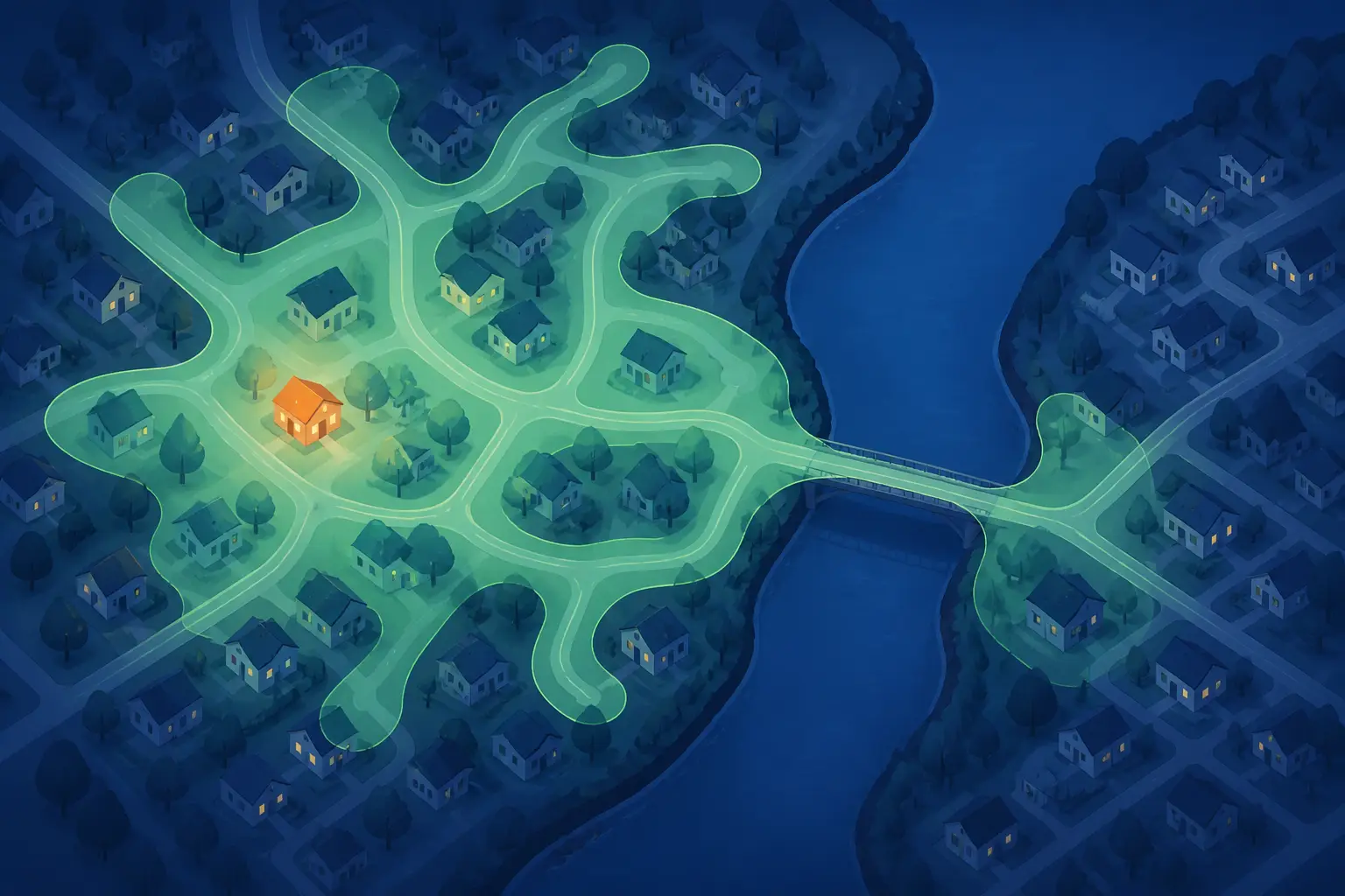
Here's the thing the local Wikipedia project got gently roasted for: it says "half-hour walk" but it actually draws a 3km crow-flies circle. A river with no bridge, a motorway, a fenced rail yard — the circle doesn't know. A genuine half-hour walk is an isochrone: the irregular blob of everything reachable in 30 minutes along the actual walking network. Two points 1km apart as the crow flies can be a 40-minute walk apart if an estuary sits between them.

Computing an isochrone means running a routing engine — OpenStreetMap data through OSRM, Valhalla, or GraphHopper — expanding a shortest-path tree from your point until travel time hits the budget, then contouring the reachable area into a polygon. That's minutes of graph preprocessing per region and tens of milliseconds per query, versus microseconds for a circle. But once you have the polygon, the containment query is just ST_Intersects, which the same spatial index handles beautifully. This is one of the cases where the spatial-index camp pulls even further ahead: polygons are a first-class citizen there, while geohash prefix tricks get genuinely awkward for arbitrary shapes (you end up covering the polygon with a set of cells — doable, Z-order and S2 libraries exist for this, but it's a project).

My honest take: for most products the circle is the right lie. Users don't audit your walking model; they notice results being fast and roughly sensible. "Within 3km" correlates well enough with "nearby" that the extra infrastructure of a routing engine is hard to justify for a content-browsing feature. The moment you're making promises with consequences — delivery ETAs, courier dispatch, emergency response coverage — the circle becomes a liability and the isochrone pays for itself. Pick the abstraction based on whether being wrong costs you money or just mild surprise.

Sourcing the Data: Geocoded Wikipedia and Address Search

If you want to build something in this spirit, the data plumbing is more approachable than people assume. Wikipedia's coordinates come from the GeoHack template system and are queryable through the MediaWiki API's list=geosearch endpoint — which is itself a radius query over a spatial index, and what the project's "Nearby" feature wraps. Wikidata's P625 (coordinate location) property covers far more than English Wikipedia if you want multilingual or non-article entities. For address lookup, the project uses Photon, an Elasticsearch-backed geocoder built on OpenStreetMap's Nominatim data — free to self-host, with a public demo endpoint that generous people run and that you shouldn't hammer in production.

One design decision worth stealing: the site keeps your location in the browser and never puts it in shareable URLs. That's the right default, and it mirrors the lesson from what fitness apps teach us about location data and OPSEC — a user's coordinates are among the most sensitive strings your app will ever hold, and the cheapest way to protect them is to never send them to your server at all. Do the geocoding client-side or via a third-party geocoder the browser talks to directly, keep only rounded coordinates if you must log anything, and your privacy posture writes itself.

For the "closest N regardless of radius" fallback, resist the urge to implement expanding-radius retry loops. PostGIS's KNN operator does it in one indexed query:

-- The closest 25 articles, whatever the distance — one query, index-ordered
SELECT title, geog <-> ST_MakePoint(:lon, :lat)::geography AS dist_m
FROM places
ORDER BY dist_m
LIMIT 25;

That single line replaces the whole "try 3km, then 6km, then 10km" retry ladder I see in so many codebases, and it's faster than one round of the ladder was.

The Recommendation

If you take one thing from this comparison, take this: start with PostGIS and a GiST index, and only reach for geohashes when your storage layer forces you to.

The reasoning is simple. The spatial index wins on median latency, wins harder on p95 in dense areas, wins on correctness (meter-accurate spheroid distances, no cell-edge bugs), wins on features (polygons, KNN, isochrone containment all become one-liners), and wins on code you don't have to write and maintain. The geohash approach requires you to correctly implement neighbor-cell computation, precision selection, and a two-phase filter — three places to be subtly wrong — to reach performance that's still worse.

Geohashes earn their place in exactly three situations: your datastore has no spatial support (DynamoDB, plain Redis, a static JSON file on a CDN), you need location-based sharding across nodes, or you're pushing the query to the client and want zero dependencies. In those cases, lean on a battle-tested library — ngeohash in Node, python-geohash, or S2 geometry if you're covering polygons — rather than hand-rolling the neighbor math.

And on the product side: ship the circle first, label it honestly ("within 3km" rather than "a half-hour walk"), make the radius configurable because rural users and city users live in different density universes, and graduate to isochrones only when the crow-flies lie starts costing you something measurable. The local Wikipedia project is a lovely reminder that the best features are often just a good spatial query wearing a friendly idea. A million articles, one index, one well-chosen radius — and suddenly the internet's largest encyclopedia feels like it was written about your street.