ZIP Code Boundaries: ZCTA vs USPS — When Each Wins
USPS now sells official ZIP code boundaries, but ZIPs were never polygons. ZCTA vs USPS boundary data: when each wins in production geocoding pipelines.
 Sarah Chen

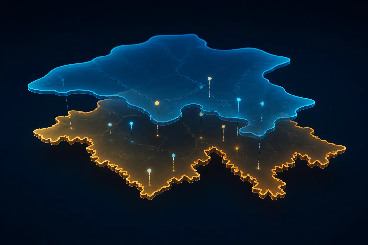
Your geocoding pipeline has a silent bug: an address in a newly built subdivision geocodes fine, then falls into the gap between two ZCTA polygons and comes back with a null region. Downstream, your delivery-cost model silently averages it into the wrong market. This is the everyday reality of working with ZIP code boundaries — a concept that, until recently, didn't officially exist at all. USPS has now started selling official ZIP Code boundary polygons through its PostalPro portal, and the data engineering world is split between excitement and sticker shock. Here's what actually changed, and how to decide which boundary data belongs in your pipeline.
I've spent years building matching and enrichment pipelines on top of US address data, and my strong opinion is this: most teams treat ZIPs as geography because the Census Bureau made it easy, not because it's correct. The new USPS product doesn't change that calculus for everyone — but it does finally settle an argument we've been having for decades.
ZIP Codes Were Never Polygons (and Still Aren't)
The fundamental fact that breaks everyone's intuition: a ZIP code is an attribute of a delivery route, not a region of land. USPS created ZIPs in 1963 to get the right mail onto the right truck. A ZIP is a collection of carrier routes anchored to a delivery unit — a post office, a sorting facility, sometimes a single building. Large receivers like government agencies and universities get their own dedicated ZIPs that cover one address. PO box-only ZIPs cover a wall of boxes inside a building and zero acres of ground.
This has consequences that polygon-thinking can't absorb. Imagine a developer builds a new neighborhood on empty land between two towns. If ZIPs were polygons, you'd look up which polygon the land sits in and that's your ZIP. Reality: USPS assigns it to whichever route makes logistical sense, which might be either town, or a brand new ZIP carved out of both. The boundary doesn't exist until the route does. That's also why USPS's own documentation says its new boundary product has temporal fluctuation — boundaries shift as delivery distribution changes, which is bureaucratic language for "routes change all the time."
- PO box and unique ZIPs have no meaningful area at all — they represent buildings, not land.
- Non-contiguous service areas happen when one delivery unit serves disconnected pockets of addresses.
- Rural gaps exist where USPS doesn't deliver at all; addresses there get assigned inconsistently, sometimes to multiple candidate ZIPs in different databases.
- Constant churn — new construction, route consolidation, and post office closures reshape the underlying routes quarterly.
- ZIP+4 narrows to a block face, but almost nobody collects or stores it, so it rarely saves you in practice.
Compare the UK, where a full postcode identifies roughly ten addresses — it was designed from the start to pin down a small group of delivery points, and it's collected and used universally. The US five-digit ZIP was designed for sorting, and we spent fifty years repurposing it for geography because it was the only geographic identifier printed on every address in the country.
ZCTA vs USPS Boundaries: What Each Dataset Actually Is
ZCTAs: Statistics Wearing a ZIP Costume
ZIP Code Tabulation Areas are the Census Bureau's answer to the polygon problem. For each decennial census, the Bureau looks at every census block, finds the most common ZIP among the addresses in that block, and groups blocks into ZCTAs named after the dominant ZIP. The result is a free, downloadable shapefile that tiles the entire country with no gaps and no overlaps.
That design has two properties that matter enormously in production. First, ZCTAs are statistical areas, built to aggregate census data consistently — every demographic table the Census publishes at ZIP level is actually ZCTA level. Second, they're lossy: the "most common ZIP wins" rule means minority addresses inside a block get assigned to a ZCTA that doesn't match the ZIP they'd write on a letter. In dense urban areas this is a rounding error. In rural areas with giant census blocks and sparse routes, a ZCTA can be off by kilometers from where any given address actually gets its mail.
The New USPS Polygons: Ground Truth, At a Price
The USPS product is built from the other direction: actual delivery address and location data, the same information that drives the trucks. That makes it the closest thing to ground truth for the question "where does USPS consider this ZIP to cover?" It ships with quarterly updates, tracking the route churn that ZCTAs lag behind. USPS sells it in three tiers — Internal, Enterprise (with limited distribution to subsidiaries and partners), and Publication (limited rights to publish derived maps).
The catch hit the community hard: pricing reportedly starts around $10,000 for the lowest tier. The anger is understandable — FCC coverage maps, federal land boundaries, and Census geography are all free, so charging five figures for postal geography feels like a step backwards. The structural reason is that USPS is a self-funding agency that largely lives off postage revenue, not congressional appropriations, so it treats data products as products. Whether that's good policy is a fair debate; whether you should build your pipeline around the licensing reality is not.
Engineering a Geocoding Pipeline for Fuzzy Boundaries
Here's the pattern I've landed on after rebuilding this pipeline more than once: treat ZIP assignment as a two-pass join with an explicit ambiguity budget, never as a single point-in-polygon lookup. The first pass is strict containment; the second pass is a capped nearest-neighbor fallback that logs itself, so you can measure how often your data disagrees with geography. This pairs naturally with the spatial indexing tricks from our geohash vs spatial index comparison — the fallback pass is exactly the kind of workload a proper R-tree makes cheap.
import geopandas as gpd
# ZCTA boundaries from the Census TIGER/Line shapefiles (free)
zcta = gpd.read_file("tl_2024_us_zcta520.shp")
# Project to a meter-based CRS so distances are meaningful
zcta = zcta.to_crs("EPSG:5070")[["ZCTA5CE20", "geometry"]]
points = gpd.GeoDataFrame(
addresses,
geometry=gpd.points_from_xy(addresses.lon, addresses.lat),
crs="EPSG:4326",
).to_crs("EPSG:5070")
# Pass 1: strict point-in-polygon
matched = gpd.sjoin(points, zcta, how="left", predicate="within")
# Pass 2: unmatched points get the nearest ZCTA, capped at 5 km,
# flagged so downstream consumers know this was an inference
unmatched = matched[matched["ZCTA5CE20"].isna()]
if len(unmatched):
nearest = gpd.sjoin_nearest(
unmatched.drop(columns=["ZCTA5CE20", "index_right"]),
zcta,
how="left",
max_distance=5_000,  # meters, because we projected first
distance_col="fallback_dist_m",
)
matched.loc[nearest.index, "ZCTA5CE20"] = nearest["ZCTA5CE20"]
matched.loc[nearest.index, "zip_inferred"] = True
matched["zip_inferred"] = matched["zip_inferred"].fillna(False)
Three details in that snippet save you from real production pain. Project to a meter-based CRS before calling sjoin_nearest — passing max_distance in degrees is a classic bug that silently means different distances at different latitudes. Cap the fallback distance: an address 40 km from the nearest ZCTA edge isn't "in" that ZCTA, it's in a data hole, and you want a null with a flag, not a confident lie. And persist the zip_inferred flag into your warehouse. When a stakeholder asks why Q3 delivery estimates drifted in Montana, that flag is the difference between a ten-minute answer and a two-week archaeology project.
Operational hygiene matters more than the join logic. Pin your boundary layer version in the pipeline config and record it as a column on output rows — when you swap ZCTA vintages or adopt the USPS layer, you need to know which boundary produced each historical record. Schedule re-ingestion to match the update cadence of your source (annual-ish for ZCTAs, quarterly for USPS), and add a validation step that diffs row counts and total area between versions; boundary files ship with data quality surprises more often than you'd hope. If you enjoy this flavor of large-scale spatial plumbing, our piece on turning a whole country into voxels covers the same lessons at a much larger scale.
A null with a flag beats a confident lie. The worst ZIP code in your database is the one that looks correct and isn't.
When Each ZIP Boundary Source Wins
The comparison isn't close once you separate use cases by what question they're actually asking. "Which ZIP does this address get mail at?" and "which statistical area does this point belong to?" sound identical and aren't.
- ZCTAs win for analytics and demographic joins. If you're enriching records with Census data — median income, population density, housing stats — ZCTAs are not just the free option, they're the correct option, because the census tables you're joining against are published at ZCTA level.
- ZCTAs win for visualization. Choropleths, market maps, and dashboards need gap-free tiling of the whole country. A boundary layer with holes where nobody gets mail looks broken to a stakeholder even when it's accurate.
- USPS polygons win for logistics and shipping. Carrier pricing zones, last-mile routing, service-area eligibility — anything where the business question is literally "what will USPS do with this address?" deserves the data built from actual delivery records.
- USPS polygons win when new construction matters. Quarterly updates track the route churn that leaves ZCTAs stale for years. If your customers build in fast-growing suburbs, this alone may justify the license.
- Neither wins when you have coordinates. If your use case is "what's near this point," skip ZIPs entirely and do real geospatial queries against lat/lon. ZIP-based proximity is a leaky abstraction.
There's also a third camp worth naming: commercial boundary vendors have sold curated ZIP polygons for years, often bundling time-series history and crosswalks to other geographies. The USPS product undercuts their ground-truth claim but not necessarily their convenience. If you already license one, the calculus is whether USPS's delivery-record lineage is worth a migration — for most analytics workloads, it isn't.

The Licensing Question Is a Dead End — Design Around It
Plenty of smart people asked whether a FOIA request could liberate this data, or whether a crowdfunding campaign could buy one license and publish the polygons. I'd bet against both. The licensing tiers exist precisely to control redistribution, and a "buy once, publish free" scheme collides head-on with the Publication tier's entire purpose. Even if it worked, you'd have a snapshot of a dataset whose value proposition is quarterly freshness — a static leak ages into a liability as routes change.
The pragmatic move is to architect so the boundary layer is swappable. Keep the join logic, the fallback behavior, and the versioning metadata constant; treat the polygon source as configuration. Then the ZCTA-to-USPS upgrade becomes a budget decision you can make per product line, not a migration project. I've seen teams hard-code ZCTA assumptions so deeply — table names, join keys, dashboard filters — that switching sources would cost more than the license they're trying to avoid.
My Recommendation: Default to ZCTAs, Buy USPS Where It Pays
Here's the decision rule I'd hand any team today. Default to ZCTAs: they're free, they tile the country, they match every census table you'll ever join, and for analytics they're the canonical choice rather than a compromise. Layer the two-pass join with a distance-capped, self-logging fallback so the seams are visible instead of silent.
Buy the USPS polygons only when the business question is about mail delivery itself — shipping cost modeling, carrier routing, service-area eligibility — and quantify the value first. Measure what fraction of your addresses land in ZCTA/USPS disagreement zones (in my experience it's low single digits nationally, but concentrated in exactly the fast-growing and rural areas where errors cost the most). If that slice drives meaningful revenue or risk, the license pays for itself; if not, you're buying precision your product can't feel.
And whatever you choose, stop pretending ZIPs are geography. They're delivery routes wearing a polygon costume, and the new official boundaries don't change that — they just make the costume better tailored. Build your pipeline to tolerate the seams, log the places where the map and the mail disagree, and you'll be ahead of most of the industry, which is still doing bare point-in-polygon lookups and wondering where the nulls come from.