Time-Series Foundation Models Make Custom Training Obsolete

Here's a claim that would have gotten me laughed out of any forecasting team five years ago: for most time-series problems, training a model on your own data is now a waste of time. A time-series foundation model — one trained on millions of series you'll never see, in domains you don't work in — will probably beat your carefully tuned pipeline, zero-shot, in the time it takes to run a single forward pass on a CPU. Mistral's Timestral, released this week in sizes from 5M to 209M parameters, is the latest and strongest evidence that this is where the field has landed. And I think a lot of practitioners are going to resist that conclusion for entirely understandable, mostly wrong reasons.

What a time-series foundation model actually is

The analogy to LLMs is useful but only if you push past the surface. A large language model is pre-trained on a huge corpus of text so that it can generalize to tasks and phrasings it has never seen. A time-series foundation model (TSFM) does the same thing with continuous signals: it's pre-trained on a massive, diverse collection of series — real and synthetic — so it learns the recurring grammar of temporal data. Trends, seasonality, regime shifts, mean reversion, noise of every flavor. When you hand it your sensor stream or your sales history, it doesn't learn from scratch; it recognizes.

That last word is the whole trick, and it explains the thing that confused me on first read: how can a model trained mostly on synthetic data beat models trained on real data? Because the synthetic generators are built to produce processes with coherent dynamics — realistic combinations of trend, seasonality, and noise, plus nonlinear dependencies between series. The model learns an enormous prior over what temporal behavior can look like. Your real series, weird as you think it is, is almost certainly some recombination of patterns it has seen a million times.

Timestral's training recipe makes this concrete. First, large-scale pre-training on purely synthetic data with a context of 8,192 time steps. Then post-training on a mix of real and synthetic data with the context stretched to 32,768 steps. The objective is a pinball loss over 21 quantiles, which means the model doesn't output a point estimate — it outputs a full uncertainty distribution, so you get a forecast with honest error bars rather than a single confident number.

One architectural detail worth stealing for your mental model: Timestral uses what Mistral calls decoupled horizon forecasting. Earlier causal decoders like TimesFM mask out the values to be forecast, which is simple but wasteful — masked values become invisible as context, so every forecast degrades the input for later forecasts. Timestral keeps the full history in the sequence and adds learned forecast tokens that read that history. Every observed value serves as both training target and context. It's the kind of small structural fix that doesn't sound dramatic and matters enormously at scale.

Zero-shot forecasting: why it beats your per-series pipeline

The strongest argument for TSFMs isn't the benchmark leaderboard — it's the shape of real forecasting work. Almost nobody forecasts one series. You forecast ten thousand. A retailer forecasts demand per SKU per store. A platform team forecasts latency per service per region. An industrial plant has thousands of sensors across hundreds of assets. The classic options are all bad: fit one ARIMA per series and watch most of them fail because each series has thin history, or train one global gradient-boosted model and drown in feature engineering and scale mismatches between series.

A TSFM sidesteps the dilemma. One checkpoint, no per-series fitting, and the cross-series knowledge is baked in from pre-training rather than having to be discovered from your data alone. This is why practitioners who actually run forecasting at scale tend to be the least skeptical of these models — the alternative isn't some elegant hand-tuned model, it's a pile of AutoARIMA jobs that take hours and silently break on the weird 5% of series that matter most.

The efficiency story is the part that surprised me most. Timestral's largest model is 209M parameters — tiny by LLM standards — and it doesn't need a GPU at inference. On a standard 8-thread server CPU, forecasting one day ahead from three weeks of 15-minute data takes 10 ms with the 5M model and 140 ms with the 209M. The 123M model lands within 0.2% of the big model's benchmark score at three-quarters of the latency. This mirrors what's happened in language models, where the interesting action has moved to small, fast tiers — the same dynamic I covered in our piece on flash-tier LLMs: the frontier model gets the headlines, the small efficient one runs the business.

And the economics compound. Ten thousand series times a daily forecast at tens of milliseconds each means your entire forecasting workload fits in a lunch break on one boring CPU box. No GPU cluster, no distributed training job, no MLOps heroics. Five years ago, building and deploying a decent forecasting model took months. Now it's an afternoon, and a big chunk of that afternoon is data plumbing, not modeling.

Covariates are the real feature, and the real catch

Here's where I'll concede ground to the skeptics, because the sharpest criticism of TSFMs is correct: for many problems, the history of the target series is a minority of the information. If you're modeling electricity demand, the weather forecast, the holiday calendar, and the pricing schedule aren't seasoning on the forecast — they are the forecast. A model that treats your carefully curated covariates as a gentle quality improvement is a model that will embarrass you precisely when the regime changes, which is precisely when you need it.

Timestral's answer is covariate-aware attention, and the design is more principled than it sounds. Every input series gets a role: target, past-only covariate, or known-future covariate. Known-future covariates — production schedules, planned shutdowns, weather forecasts — are visible across the whole window, while targets stay causal, and information flows only from covariates to targets. That last constraint is the important one: it means the model can condition on next week's scheduled load increase without leaking the target's own future into the prediction. Data leakage through covariates is one of the classic silent failures in forecasting systems, and baking the direction of information flow into the attention mask is a clean way to prevent it.

Categorical covariates get proper treatment too — a machine state like running, idle, or under maintenance is fed in as a category rather than being smashed into an arbitrary integer that imposes a fake ordering. Anyone who has watched a tree model learn that "state 3" is somehow greater than "state 2" will appreciate this.

But notice what this means in practice: the quality of a TSFM deployment is now bounded by the quality of your covariate pipelines, not your model. If your weather feed is stale, your holiday calendar is missing regional holidays, and nobody has encoded the maintenance schedule into a machine-readable form, the model can't save you. The modeling got commoditized; the data engineering did not. Budget your effort accordingly.

Benchmarks, and why you should test on your own signal

On the three main public benchmarks — GIFT-Eval, TIME, and fev-bench — Timestral's 209M model ranks first among pre-trained, zero-shot models, with a single checkpoint and no ensembling. The 28M model reportedly beats Chronos-2, which is about four times larger. Those are genuinely strong results, and the fact that every model size in the family sits on the accuracy-versus-size Pareto front suggests the recipe, not just the scale, is doing the work.

Now the necessary caveats. Forecasting benchmarks have a deep methodological problem: many of the series in them are high-noise, low-signal processes where almost any reasonable model performs about the same, because there isn't much signal to capture. If you average scores across hundreds of such series, you compress real differences into tiny margins — which is how you get marketing charts where a 0.03 improvement is drawn to look like a fivefold gap. This is a specific instance of a general disease we've written about before: benchmarks systematically miss the work that actually matters, and forecasting benchmarks miss it in a particularly quantifiable way.

The better test, and one you can run yourself, is to construct evaluation series with a known, high signal-to-noise ratio — where a simple method like empirical conditional distributions can capture most of the signal — and check whether the foundation model captures it too. Then sweep the noise level up and watch where it degrades. A model that looks SOTA on noisy benchmarks but leaves obvious signal on the table in clean regimes is telling you something the leaderboard won't.

On noisy data, every model looks the same. The models only separate when there's real signal to capture — so test where the signal is.

Where classical methods still win

My opening claim needs honest limits, so here they are. There are real cases where you should not reach for a foundation model.

• You need the equations, not just the outputs. If you're a grid operator or a control engineer, you often need an interpretable dynamical model — parameters with physical meaning you can reason about, stress-test, and hand to a regulator. A TSFM is a black box: y = F(x, params) with no readable structure. A fitted state-space or SINDy-style model gives you something a neural net never will.
• You have one critical series with rich, long history and strong domain structure. A single well-understood series — say, a national electricity load with decades of data — rewards a bespoke model built with domain knowledge. Zero-shot generality is wasted when you only have one problem and deep expertise in it.
• Your covariates dominate and your relationships are stable and known. A linear regression on the right features is transparent, debuggable, and — when the physics of the problem are genuinely linear — unbeatable. Don't pay a complexity tax for no gain.
• You must own the dependency completely. Timestral ships under a modified MIT license with restrictions, and if your forecasting is load-bearing infrastructure — day-ahead energy markets, say — you need to think hard about depending on a vendor's server or a license you can't fully control. Open-weight alternatives and in-house models exist precisely for this case.
• You have strict backtesting hygiene requirements. With a pre-trained model, you can never be fully certain your backtest period wasn't in the training corpus unless the vendor gives you control over the training mix. Mistral offers that through its Forge pipeline, but verify it rather than assuming it.

Notice the pattern: the foundation model wins on breadth, speed, and sparse data; it loses on interpretability, single-series depth, and dependency risk. That's a genuinely useful decision rule, and it's sharper than the usual "it depends."

The architecture question everyone skips

One thing the TSFM wave has settled that deserves more attention: transformers work fine on continuous signals, and the tokenization problem turned out to be less scary than expected. The trick is patching — instead of treating each time step as a token (which explodes sequence length) or embedding raw floats naively, you chunk the series into patches and embed those. Patch lengths become a tunable knob trading resolution against context, exactly like vocabulary size in an LLM. If you've followed the debate over state-space models versus transformers, it's notable that the winning TSFMs so far are mostly attention-based — the long-range structure of temporal data seems to suit attention well once you fix the input representation.

The synthetic-first data strategy deserves equal billing as a contribution. Most of Timestral's training data was generated, not collected: univariate processes with coherent dynamics first, then a multivariate synthesizer layering nonlinear dependencies between them. This neatly sidesteps the data problem that has haunted time-series ML — there's no Common Crawl of sensor data, and what exists is siloed, proprietary, and inconsistently formatted. If synthetic data with the right inductive biases transfers this well, it changes the economics of the whole subfield. You don't need to hoard the world's telemetry; you need good generators.

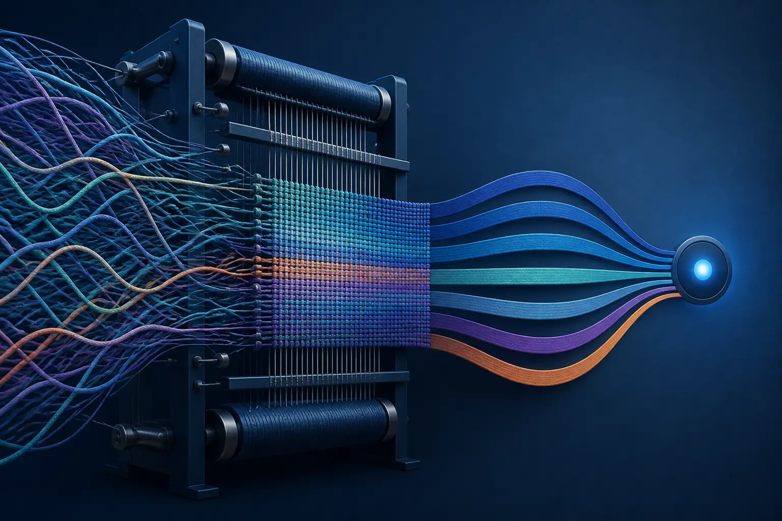
From forecast to system

The most interesting long-term consequence isn't the model — it's what the model enables downstream. A cheap, probabilistic, multivariate forecaster running continuously on your metrics is an anomaly detector with honest uncertainty: instead of alerting when a value crosses a static threshold, you alert when reality falls outside the predicted quantiles, which means alerts that respect seasonality and planned events. A scheduled load increase is expected rather than flagged as a surprise. That alone would eliminate a depressing fraction of pager noise in most organizations.

Layer an LLM agent on top and you get the workflow Mistral sketches: the numerical model flags an anomaly on a pump, an agent compares the signals against embeddings of past failures, spawns a root-cause analysis over maintenance records and operator notes, and hands the plant manager a diagnosis with evidence instead of a bare alert. Whether or not you buy that specific vision, the direction is sound — it's the same pattern we've seen with constrained decoding for decision models: keep the fast, specialized model in the loop for what it's good at, and let the general model orchestrate around it.

So here's where I land. Bespoke forecasting isn't dead — it's been demoted from the default to the specialist tool. If you have one series, deep domain knowledge, and a need for interpretable dynamics, keep fitting your state-space models and sleep well. But if you have thousands of series, thin history per series, and a team of three, the burden of proof has flipped: you now need a reason not to start with a foundation model. Test it on your own high-signal data, wire in your covariates properly, check the license against your risk tolerance — and then spend the months you saved on the data plumbing, which is where forecasting projects were always really won or lost anyway.